Visualization of multivariate functions, sets, and data
We provide visualization tools which are specialized for visualizing multivariate density functions and density estimates. Tools are also provided for visualizing multivariate data.
Multivariate functions are visualized with level set trees. Level set trees transform a multivariate function to a 1D function so that its mode structure is isomorphic to the original multivariate function. A volume plot is a plot of this 1D function and a barycenter plot shows the locations of the barycenters of the level sets.
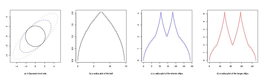
When a multivariate function is unimodal we may visualize the boundary functions of its level sets with the level set tree type methods. We call a shape tree a recursive approximation of a connected set, and a radius plot or a tail probability plot visualizes the mode structure of the boundary function. A location plot shows how the shape is located in the multivariate Euclidean space.
A discrete set may be visualized with a similar type of recursive approximation as continuous sets. We call a tail tree such a recursive approximation of a multivariate point cloud. A tail frequency plot and a tail tree plot show the mode structure of this point cloud.
We provide an R package "denpro". R is a language and environment for statistical computing and graphics. It may be downloaded from R archive network .
The package "denpro" is designed by Jussi Klemelä. I am grateful for bug reports.
Contents
Introduction:
Level set trees
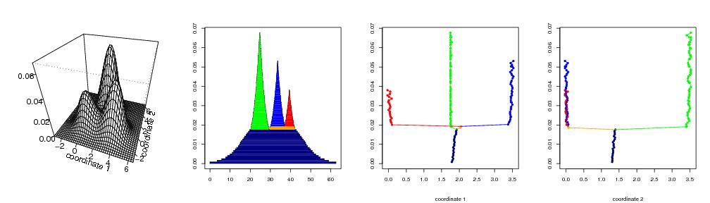
We visualize a density function with the help of its level set tree. A level set tree is a tree structure built from the separated components of the level sets of the function. It makes a recursive approximation of the function. With different graphical representations of level set trees we may visualize the number and relative importance of the modes, the barycenters of the separated regions of the level sets, in particular the locations of the modes, and the skewness and the kurtosis of the density. The visualization method may be applied in exploratory data analysis, to make graphical inference on the existence of the modes, and to apply graphical methods for the smoothing parameter selection. Visualization with level set trees is in many cases more effective and easy to use than the method of looking at slices and projections of the density function.
Studying level sets of a function for a series of levels provides information on the shape of a multivariate function. Level sets has been applied in mode detection and density estimation in 3 and 4 dimensional cases. In the 4D case one may visualize 3D density contours as the fourth variable is changed over its range. Studying projections and marginal densities is in many cases sufficient but projections may hide some high dimensional features.
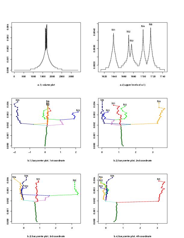
In density estimation we are interested how the probability mass is distributed over the d-dimensional Euclidean space. Local extremes of the density function express concentration of the probability mass. We are interested both in visualizing the locations of these local extremes, and also in visualizing the size of the probability mass associated with each local extreme. A volume plot visualizes the amount of probability mass associated with each local extreme. A barycenter plot visualizes the locations of these probability masses, drawing a "skeleton" of the function.
The figures below show an equal mixture of 4 Gaussian densities in the 3D Euclidean space.
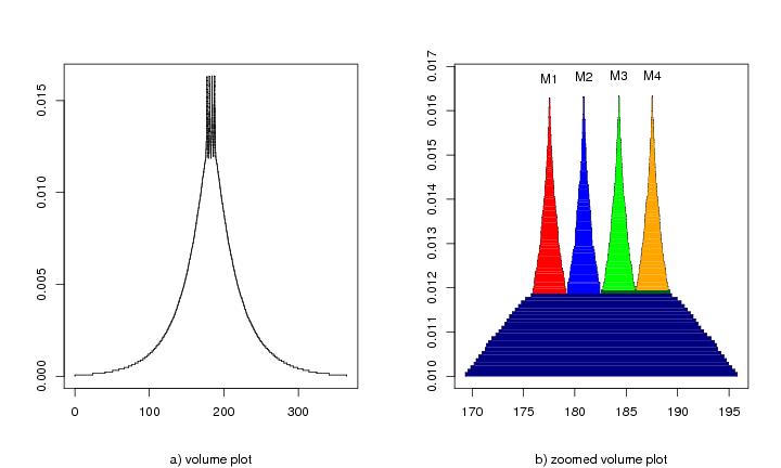
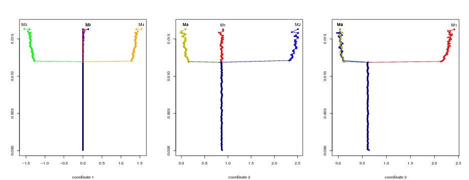
Below we visualize a kernel estimate with 2000 observations from a mixture of 5 Gaussian densities in the 4D Euclidean space. Window a.1) shows the volume plot, a.2) zooms to the upper levels of the estimate, and b.1-4) show barycenter plots.
Below we illustrate the definition of the level set tree.
Shape trees
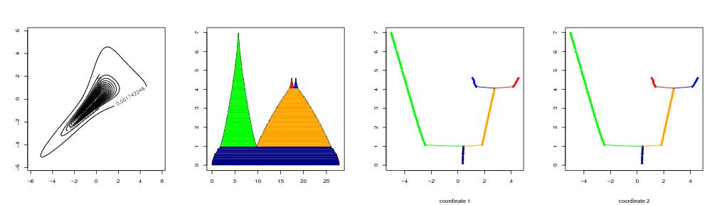
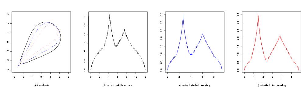
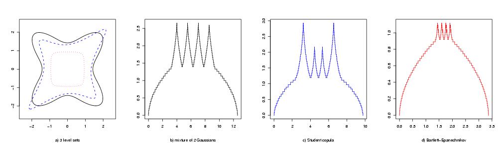
Beyond the mode structure, level set tree based plots give only a limited insight into the shape of the density. We need additional visualization tools since also unimodal densities may have a large variety of shapes: the probability mass is distributed only in some regions of the huge multivariate Euclidean space. The visualization tools which we present are based on a shape tree of a set. We visualize a density by visualizing a series of level sets of the density. We form a series of shape trees from a series of level sets and apply graphical tools to visualize the shape trees. A shape tree may be formed from a connected set, where by a connected set we mean a set which cannot be expressed as a union of two sets which do not touch each other. A shape tree of a connected set is a tree which is formed by looking at the deviations of the set from the spheres centered at a given reference point, where the reference point is typically the location of the mode of the density, or the barycenter of the set. Level sets of a unimodal density are connected. When a density is multimodal some of its level sets, possibly at higher levels, are not connected, and in this case we should visualize separately each connected component, or restrict ourselves to the visualization of lower level sets.
A shape tree of a star shaped set is basically a level set tree of its boundary function.
A shape tree of a connected set is a tree which is formed by looking at the deviations of the set from the balls centered at a given reference point, where the reference point is typically the location of the mode of the density, or the barycenter of the set. The root of the tree is identified with the set itself. The non-root nodes correspond to the separated components of the intersection of the set with the complement of a ball centered at the reference point.
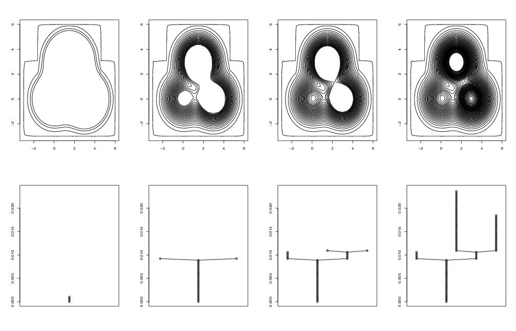
We present two types of plots: the shape plots and the location plot. The shape plots visualize only the shape of the set and the location plot visualizes spatial information showing how the shape is located in the multivariate Euclidean space. The shape plots include the radius plot, the tail probability plot, the probability content plot, and the volume plot. These plots are plots of 1D functions which are obtained from the shape tree. Thus we define transforms of a multivariate set to 1D functions. For example, a radius content transform reveals basically the following features of the set.
- Qualitative information. The modes of the radius transform correspond to the ``extensions'' or ``tails'' of the set, where with extensions of the set we mean those parts of the set which do not fit inside a given ball. We call a connected set ``multimodal'' when the radius transform is multimodal.
-
Quantitative information.
- The lengths of the level sets of the radius transform are equal to the volumes of the corresponding regions of the original set.
- The levels of the level sets of the radius transform are equal to the distance of the corresponding regions of the original set from the reference point.
Below are examples of 2D radius transforms.
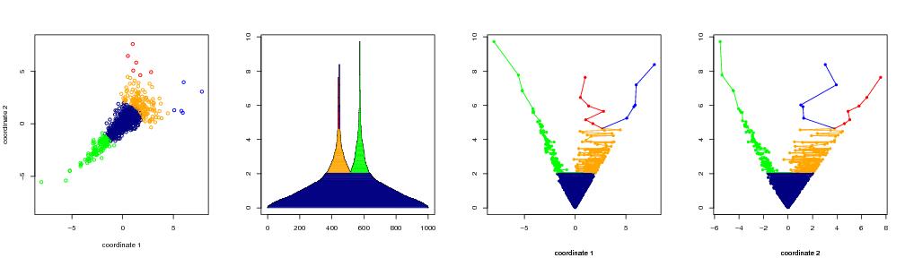
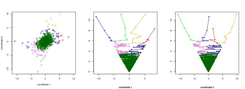
Tail trees
With tail trees we visualize the shape, the location, and the orientation of a multivariate point cloud. We interpret the point cloud as realizations of n random vectors having a common density function. We concentrate on the case where the point cloud is connected in the sense of single linkage clustering. The assumption of the connectedness of the point cloud may be interpreted as the connectedness of the support, or a low-level level set, of the density which has generated the observations.
The visualizations are based on the concept of a tail tree of a set. A tail tree of a set of finite cardinality is a tree whose nodes are associated with the subsets of the set, so that the sets in the upper levels of the tree correspond to the extensions or tails of the set. The concept of a tail tree is closely related to the concept of a shape tree. A shape tree is defined for a connected set, when the connectedness was defined in terms of the topology of the Euclidean metric. We want to modify that concept in order to visualize sets of finite cardinality. A shape tree may be applied to visualize level sets of a density estimate, but with tail trees we may visualize the raw data, avoiding the density estimation step. Since density estimation is difficult in high dimensional cases we may be able to analyze higher dimensional data with tail trees than with shape trees.
Below we visualize a data of size 1000 from a distribution with Gaussian copula whose shape parameter is r=0.5, and whose marginals are Student with degrees of freedom 3.
Literature:
Level set trees are described in the article "Visualization of multivariate density estimates with level set trees" . See Homepage of the article .
Shape trees are described in the article "Visualization of multivariate density estimates with shape trees" .
Some algorithms related to level set trees are described in the article "Algorithms for manipulation of level sets of nonparametric density estimates". The article describes algorithm DynaDecompose, but please note that algorithm LeafsFirst is now better supported.
Tail trees are described in the article "Visualization of multivariate data with tail trees" .
Some 2D shape isomorphic transforms (2D volume function and 2D probability content function) are described in the article "Visualization of the spread of multivariate distributions".
Mode graphs and branching maps are described in the article "Visualization of scales of multivariate density estimates".
Installation instructions:
The programs are provided as an R-package. There are two ways to install the functions.
-
Download the file denpro.R and then issue the command
> source("/path/denpro.R")
in the R console. Note that one has to specify the full name of the file and use for example in Unix the command
> source("/home/aaa/Desktop/denpro.R")
where "aaa" is the user account, in OS X
> source("/Users/aaa/Desktop/denpro.R")
and in Windows XP
> source("C:\\Documents and Settings\\user\\Desktop\\denpro.R")
-
Download package denpro_0.9.2.tar.gz
-
Windows and X OS binaries are available at http://www.r-project.org/ (-> CRAN -> Choose mirror -> Packages)
-
Installation instructions are provided by issuing command R CMD INSTALL --help or command R INSTALL --help. Installation may be done (in unix) with the command:
R CMD INSTALL denpro_0.9.0.tar.gz
For example, in Ubuntu the package will be in directory /usr/local/lib/R/site-library/denpro/ and in Suse the package will be in directory /usr/lib/R/library/denpro/
-
In R, issue the command
library(denpro)
which makes the functions available.
-
Documentation:
Here is a listing of the functions, which the package provides.
Functions to calculate a level set tree, shape tree or tail tree:
- leafsfirst : computes a level set tree or a shape tree from a piecewise constant function with the "LeafsFirst" algorithm, computes a tail tree from a data matrix
- leafsfirst.adagrid : computes a level set tree of a discretized kernel estimator with an adaptive grid; the function is applied to the output of function "pcf.greedy.kernel", which belongs to package "delt"
- leafsfirst.intpol : computes a level set tree from a function evaluated at any set of points
- plotvolu : draws a volume plot of a level set tree, a radius plot, tail probability plot, or probability content plot of a shape tree, and a tail frequency plot of a tail tree.
- plotbary : draws a barycenter plot of a level set tree, a location plot of a shape tree, and a tail tree plot of a tail tree.
- plottree : draws a tree plot from a level set tree, shape tree, or tail tree
- treedisc : prunes a shape tree, level set tree or a tail tree to have fewer levels
- treedisc.intpol : prunes a level set to have fewer levels, when the level set tree is calculated with function "leafsfirst.intpol"
- prunemodes : prunes the smallest modes (in terms of the excess mass) away from a level set tree or a shape tree
- leafsfirst.intpol.volu : computes the volumes of level sets after calculating the level set tree with function "leafsfirst.intpol"
Visualization of scales of estimates:
- lstseq.kern : computes a sequence of level set trees of kernel estimates corresponding to a scale of smoothing parameter values; applies programs "pcf.kern" and "leafs.first" consecutively
- modegraph : computes a mode graph from a sequence of level set trees
- plotmodet : plots a mode tree
- branchmap : computes a a branching map from a sequence of level set trees
- plotbranchmap : plots a branching map
- scaletable : plots a scale and shape visualization table
- exmap : computes a scale of excess mass profiles from a sequence of level set trees
- plotexmap : plots a scale of excess mass profiles
- hgrid : returns a vector of smoothing parameters with logarithmic spacing
Visualization of anisotropic spread (2D volume function and 2D probability content function):
- stseq : returns a sequence of shape trees, corresponding to a scale of levels
- shape2d : makes a 2D volume function or 2D probability content function
- plotvolu2d : plots a 2D volume function or 2D probability content function
- plotdelineator: plot the locations of the delineators of a sequence of sets; the locations correspond to the modes of the 2D volume function or probability content function
Other utilities:
- pcf.kern : computes a kernel density estimate; the estimate is returned as a piecewise constant function
- kernesti.dens : computes a kernel density estimate at a single point
- pcf.histo: computes a histogram estimate; the estimate is returned as a piecewise constant function
- draw.pcf : returns the matrix of values of a 2 dimensional piecewise constant function; this data is given as an input to programs "persp" or "contour" to draw a picture of the function
- draw.levset : draws a level set of a 2 dimensional piecewise constant function
- tree.segme : returns the segmentation of the nodes of a visualization tree
-
Calculation of level set trees with "DynaDecompose" algorithm
and with naive algorithm
- profkern : computes a level set tree of a kernel estimate with the "DynaDecompose" algorithm
- profhist : computes a level set tree of a histogram with the naive algorithm
- profgene : computes a level set tree of a rectangularwise constant function with the naive algorithm
- profeval: computes a level set tree of a function given in the evaluation tree format. Applies DynaDecompose algorithm. The function is not supported.
- locofmax : returns the location of the maximum of a piecewise constant function
- modecent : returns the locations of the modes (local maxima) of a function represented with a level set tree
- excmas : function to return excess masses associated with the nodes of a level set tree
- lst2xy: transforms a level set tree or a shape tree to vectors x and y to be plotted by the command plot(x,y)
Other visualization tools:
- slicing : returns a one- or two-dimensional slice of a piecewise constant function
- paracoor : makes a parallel coordinate plot
- paracoor.dens : makes a parallel coordinate density plot
- graph.matrix: plots a graphical matrix in the sense of Bertin, where the permutation with respect to observations is given by a tail clustering of the data.
- plotbary.slide: makes a slide show of the d windows of a barycenter plot, location plot, or tailtree plot.
- pp.plot: makes a PP-plot
- qq.plot: makes a QQ-plot
- plot.kernscale: plots a scale of 1D kernel estimates
- paraclus: parallel level plots of clusters
- dist.func: plots a 1D distribution function
Clustering:
- colors2data : assigns colors to data points according to cluster membership, when the clusters are defined as high density regions
- finbnodes : finds pointers to the nodes of a level set tree; the nodes are such that their excess mass is among "modenum" largest excess masses, and they start a new branch.
Miscallenous:
- pcf.func : returns piecewise constant functions of certain parametric forms, for example mixtures of Gaussians, skew Gaussians, densities with Clayton copula, Plackett copula.
- sim.data : simulates data for some examples
- dend2parent: makes a tree with parent-links from a dendrogram object
- explo.compa: given a data set, generates a Gaussian data of the same size, with the same mean vector and the covariance matrix as the original data
- nn.radit: finds for each observation the distances to the k nearest neigbors
- nn.likeset: finds a subset of a data matrix with likelihood subsetting; a nearest neighbor density estimator is used
- rotation: returns a rotation matrix for a given angle
- liketree: computes a likelihood tree of the observations
- leafsfirst.visu: illustration of the leafsfirst algorithm (level set trees)
- plottwin: illustration of the leafsfirst algorithm (shape trees)
- histo1d: computes and draws an 1D histogram estimate
- perspec.dyna: makes a dynamic perspective plot
- point.eval: returns the value of a function at a point, when the function is represented as an evaluation tree
- preprocess: preprocessing of the data matrix; either sphering or the copula preprocessing
In R use the command help(func) to get online manual for "func".
Tutorial:
# First load the library

library(denpro)
Short tutorial
# level set tree

dendat<-sim.data(n=200,type="mulmod")   # data
pcf<-pcf.kern(dendat,h=1,N=c(32,32))    # kernel estimate

lst<-leafsfirst(pcf)             # level set tree
td<-treedisc(lst,pcf,ngrid=60)   # pruned level set tree

plotvolu(td)                     # volume plot

plotbary(td)                     # barycenter plot

# shape tree

dendat<-sim.data(n=200,type="cross")    # data
pcf<-pcf.kern(dendat,h=1,N=c(32,32))    # kernel estimate

st<-leafsfirst(pcf,propo=0.01)   # shape tree, 1 per cent level set
tdst<-treedisc(st,pcf,ngrid=60)  # pruned shape tree

plotvolu(tdst)          # radius plot

plotbary(tdst)          # location plot

# tail tree

dendat<-sim.data(n=200,type="cross")    # data

tt<-leafsfirst(dendat=dendat,rho=0.65) # tail tree

plotbary(tt)     # tail tree plot

plotvolu(tt)     # tail frequency plot
Level set trees
dendat<-sim.data(n=200,type="mulmod")   # data

# calculate a kernel estimate

h<-1                      # smoothing parameter
N<-c(8,8)                 # size of the grid
pcf<-pcf.kern(dendat,h,N) # kernel estimate as a piecewise constant function

# calculate a level set tree of the estimate

lst<-leafsfirst(pcf)

# plot a volume plot, with colors and labels

plotvolu(lst, colo=TRUE, modelabel=TRUE, ptext=0.002)

# plot a barycenter plot, for the second coordinate,
# with labels, and return the locations of the modes

plotbary(lst,coordi=2,modlabret=T,ptext=0.002)

# prune the level set tree to contain only 10 levels

td<-treedisc(lst,pcf,ngrid=10)

plotvolu(td)

# look at the contour and perspective plots of the estimates

dp<-draw.pcf(pcf)

contour(dp$x,dp$y,dp$z,xlab="coordinate 1", ylab="coordinate 2")

persp(dp$x,dp$y,dp$z,phi=20,theta=50)
Level set trees with data based interpolation
The function "leafsfirst" computes a level set tree from a piecewise constant function and the piecewise constant function is such that the pieces where the function is constant are rectangles. In high dimensional spaces regular equispaced partitions have a huge size and it might be difficult to find a good irregular partition of a reasonable size. Thus we have implemented a function "leafsfirst.intpol" that does not require an initial step of calculating a piecewise constant function but that requires only that the function is evaluated at any irregular collection of points. The basic examples where we can use this function are a density function estimate that is evaluated at the observations, and a regression function estimate that is evaluated at the observations of the x-variables.
Function "leafsfirst.intpol" approximates level sets of the function with unions of balls, centered at the points where the function is evaluated. Thus we have to provide the radius of the balls (parameter rho). The choice of parameter rho affects the level set trees, because a too small parameter rho results to a level set tree with many spurious local maxima and a too large parameter rho results to a level set tree with only one local maxima.
source("denpro.R")

# simulate data "dendat"
n<-200
dendat<-sim.data(n=n,type="mulmod")

# kernel density estimate is evaluated at the observations
f<-matrix(0,n,1)
h<-0.4            # smoothing parameter
for (i in 1:n){
  arg<-dendat[i,]
  f[i]<-kernesti.dens(arg,dendat,h)
}

# calculate a level set tree with level sets that are
# collections of balls of radius rho=0.6
rho<-0.6
lst<-leafsfirst.intpol(dendat, f, rho=rho)

# plot a level set tree and a volume plot of the level set tree
plottree(lst,modelabel=FALSE)
plotvolu(lst,modelabel=FALSE)

# improve the level set tree by calculating volumes of level
# sets more accurately
M<-100       # sample size of the Monte Carlo samples
grid<-3      # the number of level sets whose volumes are calculated
lst2<-leafsfirst.intpol.volu(lst, dendat, rho, M=M, grid=grid)
plotvolu(lst2,modelabel=FALSE)

# to make plotting faster, we can prune the level set
ngrid<-40
lst.redu2<-treedisc.intpol(lst2, f, ngrid=ngrid)
plotvolu(lst.redu2,modelabel=FALSE)
Shape trees
dendat<-sim.data(n=200,type="cross")    # data
pcf<-pcf.kern(dendat,h=1,N=c(32,32))    # kernel estimate

# calculate a shape tree, when the reference point is the mode,
# and the level set corresponds to the 10 per cent level

st<-leafsfirst(pcf,propor=0.1)

# prune the shape tree

std<-treedisc(st,pcf,ngrid=60)

# plot a volume plot, with colors and labels

plotvolu(std, colo=TRUE, modelabel=TRUE, ptext=0.1, symbo="L")

# plot a barycenter plot, for the second coordinate,
# with labels, and return the locations of the modes

plotbary(std, coordi=2, modlabret=T, ptext=0.1, symbo="L")

# choose the reference point to be the barycenter

bary<-st$bary
st<-leafsfirst(pcf,propor=0.1,ref=bary)

std<-treedisc(st,pcf,ngrid=60)

plotvolu(std)
Level set trees: Kernel estimate with the DynaDecompose algorithm
dendat<-sim.data(n=200,type="mulmod")
h<-1
N<-c(32,32)
Q<-30
pd<-profkern(dendat,h,N,Q)

plotvolu(pd)

plotbary(pd,coordi=1)

plotbary(pd,coordi=2,modlabret=T)

modecent(pd)
Tail trees
# generate the data

dendat<-sim.data(n=500,type="cross")

# calculate a tail tree

rho<-0.65    # resolution threshold
tt<-leafsfirst(dendat=dendat,rho=rho)

# tail tree plots

plotbary(tt)

plotbary(tt, coordi=2, modelabel=TRUE, modlabret=TRUE, ptext=0.2, symbo="T")

# tail frequency plot

plotvolu(tt,colo=TRUE)                      # with colors

plotvolu(tt,ptext=0.2,modelabel=TRUE,symbo="T",colo=TRUE)  # with mode labels
Data structures of the package
In order to help to apply the functions of the package to visualize some user defined functions we describe some basic objects of the package.
Level set tree object
Level set tree object represents a level set tree. This object is given as an input for the visualization functions "plotvolu" and "plotbary".
Level set tree object is a list containing vectors "parent", "level", "volume" and matrix "center". Length of vectors is equal, let us call this length "nodenum". The matrix "center" is d*nodenum-matrix, where d is the dimension of the underlying function which is represented by the level set tree.
Elements of the vectors (and columns of the matrix) correspond to the nodes of the level set tree, which in turn correspond to disconnected components of the level sets of the underlying function.
- parent: describes the tree structure by giving the parent node for every node. For root nodes contains 0.
- level: gives the level of the corresponding level set.
- volume: gives the volume of the corresponding disconnected component of a level set.
- center: columns give the barycenters of the corresponding disconnected components of level sets.
Shape tree object
Shape tree object represents a shape tree. This object is visualized with the functions "plotvolu" and "plotbary".
Shape tree object is similar to the level set tree object, but the list contains in addition the vector "refe" and the real value "maxdis".
- refe: this is the reference point which was given as an argument in calculating the shape tree with the "leafsfirst" function.
- maxdis: the maximum distance from the reference point, of the rectangles forming the set.
Piecewise constant function object
The piecewise constant function object represents a rectangularwise constant function. This object is given as an input to the function "leafsfirst" which computes the level set tree with the Leafsfirst algorithm.
The piecewise constant function object is a list whose elements are vectors "value", "N", and "support", and matrices "down" and "high". The basic idea is that we have a fine regular partition and the function is piecewise constant on a non-regular partition, whose members are unions of the rectangles in the smallest resolution level. There are N[1]* … *N[d] small rectangles.
- N: d-vector of integers ≥ 1; gives the number of rectangles for each dimension.
- value: vector of real values; gives values of the function for each rectangle.
- down: M*d-matrix of integers, where M is the number of rectangles where the function is constant and d is the number of dimensions; i:th row of "down" gives the lower vertex of the i:th rectangle and in the j:th column the values of the matrix "down" are in the range 0, … ,N[j]-1.
- high: M*d-matrix of integers; i:th row of "high" gives the upper vertex of the i:th rectangle and in the j:th column the values of the matrix "high" are in the range 1, … ,N[j]. For example, rectangle [I1,J1]* … *[Id,Jd] is represented in the i:th row of "down" as [I1,…Id] and in the i:th row of "high" as [J1,…Jd]. We have that 0 ≤ I1< J1 ≤ N[1],…,0 ≤ Id < Jd ≤ N[d].
- support: d-vector of reals; defines the rectangle where the function is defined. For example, if the support of the function is rectangle [a1,b1]*…*[ad,bd], then "support" is vector [a1,b1,…,ad,bd].
In package "delt" function "pcf.greedy.kernel" computes a piecewise constant function which uses a more adaptive partition than a partition which can be obtained as combining rectangles in a regular partition. In this case the piecewise constant function is a list with elements
- value: as before
- down: pointers to "grid"
- high: pointers to "grid"
- grid: M*d matrix which contains the possible split points and boundaries
- support: as before
- recs: L*(2d) matrix which contains pointers to the rows of "grid"; defines the rectangles in the adaptive partition. For example, in dimension d=2, the row (a1,a2,b1,b2) of "recs" specifies the rectangle [grid[a1],grid[a2]] × [grid[b1],grid[b2]].
Evaluation tree object
An evaluation tree is a binary tree which stores the values of the function which have been evaluated on a grid (regular or irregular). A level set tree is a representation of the function, but how to calculate this representation when we know only how to evaluate the function at individual points? The package contains function "profeval" which computes a level set tree when the function is represented as an "evaluation tree". Note an alternative and computationally inefficient way to calculate a level set tree implemented by the function "profgene".
An evaluation tree is a binary search tree, thus making the updating fast. It stores spatially close points so that they are close in the tree structure, making calculation of a level set tree feasible, since we may apply a bottom-up dynamic programming algorithm to find the disconnected components of the level set tree.
The evaluation tree object is a list containing vectors and matrix "left", "right", "parent", "low" (matrix), "upp" (matrix), "split", "direc", "mean" "infopointer" (not implemented), "value", "down" (matrix), "high" (matrix), "support", "N", "nodefinder" (not implemented).
-
Vectors "left", "right", "parent", "split", "direc", "mean", "infopointer"
give information which is annotated to the nodes of the binary tree.
Their length is equal to the number of nodes of the binary tree.
We annotate for each node a rectangle of the underlying grid.
Matrices "low" and "upp" determine this rectangle for each node.
- "left" contains pointers to the left child, in the leafs we have 0
- "right" contains pointers to the right child, in the leafs we have 0
- "split" gives the splitting point; integer valued; in the j:th direction we have 1<= split <= N[j], in the leafs we have NA
- "direc" gives the splitted variable; integer valued; we have 1 <= direc <= d, in the leafs we have NA
- "mean" gives the value of the function at the leaf nodes; real valued
- "low" gives the lower vertices of the current rectangle, see the definition of "down"
- "upp" gives the upper vertices of the current rectangle, see the definition of "high"
- "infopointer" gives a pointer from the nodes to the rectangles, information exists only for the leaf nodes, for the other than leaf nodes 0 is stored
-
Vectors "value" and "nodefinder" and matrices "down", "high" store
the information annotated with the leafs of the binary tree.
- "value", "down", "high", "N", and "support" are as in the piecewise constant function object.
- "nodefinder" contains the pointers from the rectangles back to the leafs of the binary tree